Chi-Square Made Simple: When to Use It, How to Read It, and How to Write It Up

There is a particular kind of academic irritation reserved for tests that are not actually that complicated but are taught as though they were secret rituals. Chi-square is one of them. Students hear the name, see a Greek symbol, notice a table full of categories, and immediately assume something terrible is about to happen.

In reality, chi-square is much less dramatic than it sounds. It is usually just a way of asking whether the pattern you observed in categorical data looks different enough from what you would expect by chance to count as evidence of a real association or mismatch. That is all. Not mystical. Not elegant. Just useful.

Most first-year confusion comes from two things. First, students are not always clear on what categorical data means. Second, nobody tells them early enough that there are really two common chi-square jobs. One is checking whether two categorical variables are related. The other is checking whether one categorical variable fits an expected pattern. Once you grasp that split, the test becomes much less theatrical.

TL;DR

Use chi-square when your data are in categories, not when you are comparing means. If you want to know whether gender is associated with voting preference, or whether observed frequencies differ from what you expected, chi-square is in the right neighbourhood. If you are comparing average anxiety scores between groups, you are looking for a different test entirely.

The two versions students actually need

The first version is the chi-square test of independence. This is the one you use when you have two categorical variables and want to know whether they are associated. For example, is there a relationship between treatment condition and pass/fail outcome? Or between gender category and preference category? The test compares the counts you actually observed with the counts you would expect if the two variables were independent.

The second version is the chi-square goodness-of-fit test. This is what you use when you have one categorical variable and want to know whether the observed frequencies match some expected distribution. For example, if you expected equal numbers of responses across four categories and the observed pattern looks suspiciously lopsided, this is the version you want. Penn State’s statistics materials explicitly frame the goodness-of-fit version as testing whether observed categorical counts match an assumed model, while the independence version compares two categorical variables.

That is the first decision point. Are you testing association between two variables, or fit against an expected pattern? If you get that right, you are already ahead of a surprising number of students who are bravely clicking buttons in SPSS and hoping statistics will forgive them.

What chi-square is actually doing

Chi-square works with frequencies, which means counts. Not means. Not standard deviations. Not scores on a scale treated as continuous. It asks whether the gap between what you observed and what you expected is larger than chance would usually produce. The larger that mismatch becomes, the larger the chi-square statistic gets.

For a test of independence, the expected counts are calculated from the row and column totals as though the variables were unrelated. If the observed table looks close to that expected pattern, there is probably no meaningful association. If it looks far enough away, the test may turn significant. Penn State’s worked examples make this logic very plain by showing both the observed table and the expected count table side by side.

This is also why chi-square is so useful in psychology and social science. A lot of student projects produce categorical outcomes. Preferred option, yes/no response, diagnosis category, condition membership, pass/fail, response type. Not every dataset arrives wearing the clothes of a t-test.

The mistake students make most often

They use chi-square on data that are not really suited to it.

If your variable is genuinely categorical, fine. If it is continuous, such as reaction time, depression score, or test performance, chi-square is usually the wrong tool unless you have deliberately converted the scores into categories, which often costs you information. There are times when categorising makes sense, but students often do it because they are trying to force the data into a test they half-remember rather than choosing the test that actually fits the data.

This is one of those statistical moments where the test does not rescue the design. It merely reveals what sort of design you had.

The assumptions people forget

Chi-square is often introduced as the easy non-parametric one, which makes students think it has no real assumptions. It does. They are just less glamorous.

First, your observations should be independent. One person should not be counted multiple times in the same analysis unless the design explicitly allows for that and the method has changed accordingly. Second, the data should be counts in categories. Third, the expected frequencies should not be too small. A common teaching rule is that expected cell counts should generally be 5 or higher for the chi-square approximation to behave well. UCLA’s statistical guidance states this plainly and points students toward Fisher’s exact test when expected counts are too low, especially in small 2 × 2 tables. Penn State’s materials make the same point about the approximation working best when the cells contain a reasonable number of observations.

That expected-count issue matters more than students often realise. A chi-square test can look official while quietly resting on a table too sparse to trust. Statistics has a real talent for letting people sound confident a little ahead of their evidence.

How to read the output without panicking

Most outputs will show you the chi-square statistic, the degrees of freedom, and the p-value. For a test of independence, the degrees of freedom come from the size of the contingency table. For a goodness-of-fit test, they depend on the number of categories being compared. A significant p-value suggests the pattern is unlikely under the null hypothesis. It does not tell you that the association is large, important, or conceptually interesting. It only tells you that it is statistically unlikely to be random under the model being tested.

This is where students sometimes become p-value enthusiasts in the worst possible sense. They see p < .05 and start behaving as though nature itself has signed a confession. Calm down. The test tells you there is evidence of a discrepancy or association. You still need to think about what that discrepancy actually is.

What about effect size?

This is the part many undergraduate write-ups leave out, even though it helps answer the question the p-value does not. How strong is the association?

For chi-square tests, common effect size measures include phi (φ) for 2 × 2 tables and Cramér’s V for larger contingency tables. These help quantify the strength of the relationship rather than just its statistical detectability. Guides on chi-square reporting and effect sizes consistently note that phi is used for 2 × 2 tables, while Cramér’s V is the more general measure for larger tables.

This matters because with a large enough sample, even a tiny and fairly uninteresting association can come out significant. A proper write-up should not act as though significance and substance are the same thing. They are not. They are just very good at impersonating each other when students are tired.

A basic write-up formula

For a chi-square test of independence, a simple APA-style sentence might look like this:

A chi-square test of independence was conducted to examine the relationship between treatment condition and pass/fail outcome. There was a significant association between the variables, χ²(1, N = 120) = 6.84, p = .009, φ = .24.

If the result is not significant, you simply report that instead:

There was no significant association between the variables, χ²(2, N = 98) = 1.73, p = .421, Cramér’s V = .13.

The important thing is the order. Name the test, state the purpose, report the statistic, degrees of freedom, sample size where relevant, p-value, and, where appropriate, an effect size. UCLA’s statistical writing materials are very clear on one broader principle that applies here too: descriptive material should not be padded with unnecessary p-values, and inferential results should be reported as actual inferential findings rather than vague numeric debris.

The real point

Chi-square is one of those tests that looks more alien than it is. Once you realise it is mostly about comparing observed counts to expected counts, it stops being an occult symbol and starts being a fairly blunt question: is this pattern weird enough that chance alone is a poor explanation?

That is useful. More useful, frankly, than the way it is often taught.

A lot of first-year statistics anxiety comes from being shown tests as isolated names rather than as answers to practical questions. Chi-square makes much more sense once you stop treating it as a formula to memorise and start treating it as a match between categorical data and a question about association or fit. At that point, the Greek letter becomes much less threatening and the actual thinking becomes much easier.

Stop Guessing Your Chi-Square Write-Up

If you have ever stared at a contingency table and wondered whether you need a chi-square test, a Fisher’s exact test, a goodness-of-fit test, or divine intervention, that is exactly the sort of problem the Original Matter Stats Pack is built for.

It includes the Stats Test Advisor to help you narrow down the right test for the job, and the Chi-Squared Calculator to help you organise observed and expected counts, check the main output clearly, and generate a cleaner APA-style write-up for psychology and social science assignments. The broader pack also helps with descriptive statistics, sample size, effect size, and regression assumptions, which is useful if your statistical problems have started arriving in groups.

Because the point of the assignment is usually the research question. Not the part where you spend forty minutes trying to remember whether chi-square was the one with means, medians, or categories.

Our Tools in Action

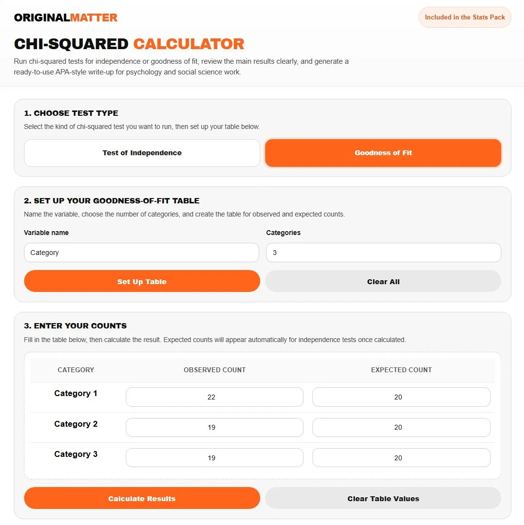
Let’s see if a six-sided die is weighted. In this case, we roll a die 60 times, then use three categories to represent rolling a 1 or 2, a 3 or 4, and a 5 or 6. If the die is fair, each category should have the same count.

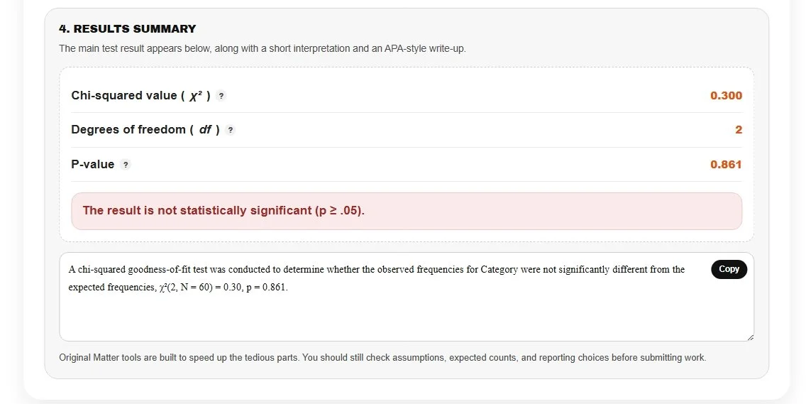
Because your p (0.861) is much greater than the standard alpha level of 0.05, we fail to reject the null hypothesis. This confirms that there is no statistically significant difference between your observations and a fair distribution, we have fair die and you have a ready to go APA style write up!

References

Ferguson, C. J. (2009). An effect size primer: A guide for clinicians and researchers. https://sdan.sites.umassd.edu/files/2023/01/An-Effect-Size-Primer-A-Guide-for-Clinicians-and-Researchers.pdf

Penn State Eberly College of Science. (n.d.). 8 chi-square test for independence. STAT 500. https://online.stat.psu.edu/stat500/Lesson08.html

Penn State Eberly College of Science. (n.d.). 2 binomial and multinomial inference. STAT 504. https://online.stat.psu.edu/stat504/Lesson02.html

Penn State Eberly College of Science. (n.d.). 4 tests for ordinal data and small samples. STAT 504. https://online.stat.psu.edu/stat504/Lesson04.html

University of California, Los Angeles, Institute for Digital Research and Education. (n.d.). What statistical analysis should I use? Statistical analyses using SPSS. https://stats.oarc.ucla.edu/spss/whatstat/what-statistical-analysis-should-i-usestatistical-analyses-using-spss/

University of California, Los Angeles, Institute for Digital Research and Education. (n.d.). Statistical writing. https://stats.oarc.ucla.edu/other/mult-pkg/seminars/statistical-writing/

University of North Texas. (n.d.). Chapter 12: Chi-square tests of independence and homogeneity. https://sites.geography.unt.edu/~wolverton/ChiSquare.pdf